library(ISLR)해당 자료는 전북대학교 이영미 교수님 2023응용통계학 자료임
Data
Credit Card Default Data :
A simulated data set containing information on ten thousand customers. The aim here is to predict which customers will default on their credit card debt.
default : A factor with levels No and Yes indicating whether the customer defaulted on their debt
student : A factor with levels No and Yes indicating whether the customer is a student
balance : The average balance that the customer has remaining on their credit card after making their monthly payment
income : Income of customer
head(Default)| default | student | balance | income | |
|---|---|---|---|---|
| <fct> | <fct> | <dbl> | <dbl> | |
| 1 | No | No | 729.5265 | 44361.625 |
| 2 | No | Yes | 817.1804 | 12106.135 |
| 3 | No | No | 1073.5492 | 31767.139 |
| 4 | No | No | 529.2506 | 35704.494 |
| 5 | No | No | 785.6559 | 38463.496 |
| 6 | No | Yes | 919.5885 | 7491.559 |
plot(Default$balance, Default$income,type='n',
    xlab='Balance',
     ylab = 'Income',
     cex.axis = 0.8)
points(Default[Default$default=='No',]$balance,
        Default[Default$default=='No',]$income,col='steelblue')
points(Default[Default$default=='Yes',]$balance,
        Default[Default$default=='Yes',]$income,col='darkorange', pch=3)

legend("topright", c("Default = Yes", "Default = No"),
        col=c('darkorange', 'steelblue'),
        pch = c(3,1),
        # bty = "n",
        cex=0.7)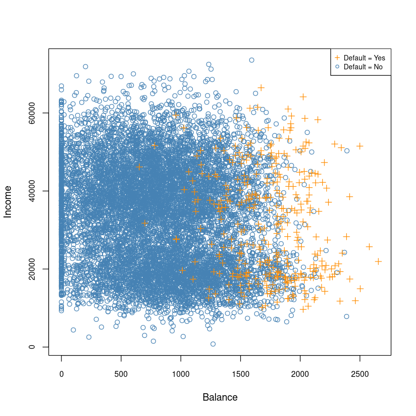
- Balance와 Income은 상관관계가 없어 보인다.
par(mfrow=c(1,2))
boxplot(balance~default, data=Default,cex.axis = 0.8,
           xlab = 'Default', ylab='Balance', col=c('steelblue', 'darkorange'))
boxplot(income~default, data=Default,cex.axis = 0.8,
         xlab = 'Default', ylab='Income', col=c('steelblue', 'darkorange'))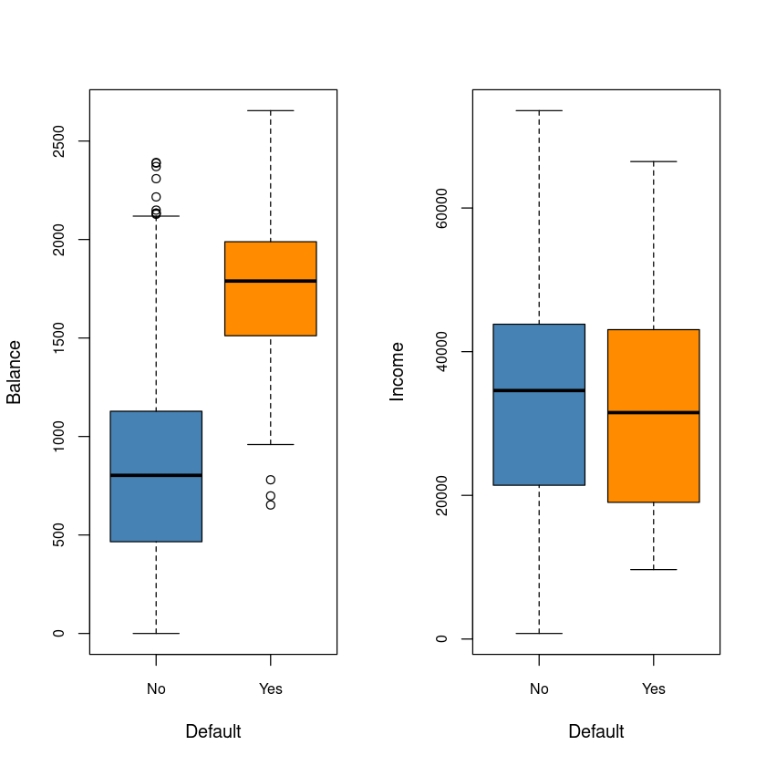
- income은 default와는 관계가 없어보인다.
Logistic regression
ordinary linear model : \(y = β_0 + β_1x + ϵ\)
Logistic Regression model
\[ log \left( \dfrac{p(y=1|x)}{p(y=0|x)} \right) = log \left( \dfrac{p(x)}{1-p(x)} \right) = \beta_0 + \beta_1 x\]
- 단순선형회귀모형
lm.fits <- lm(as.numeric(default)-1 ~ balance,data = Default)
summary(lm.fits)
Call:
lm(formula = as.numeric(default) - 1 ~ balance, data = Default)

Residuals:
     Min       1Q   Median       3Q      Max
-0.23533 -0.06939 -0.02628  0.02004  0.99046

Coefficients:
              Estimate Std. Error t value Pr(>|t|)
(Intercept) -7.519e-02  3.354e-03  -22.42   <2e-16 ***
balance      1.299e-04  3.475e-06   37.37   <2e-16 ***
---
Signif. codes:  0 ‘***’ 0.001 ‘**’ 0.01 ‘*’ 0.05 ‘.’ 0.1 ‘ ’ 1

Residual standard error: 0.1681 on 9998 degrees of freedom
Multiple R-squared:  0.1226,    Adjusted R-squared:  0.1225
F-statistic:  1397 on 1 and 9998 DF,  p-value: < 2.2e-16
y가 0 또는 1의 값인데 numeric으로 하면 1,2로 나와서 -1로 빼줌
모형 유의하지만 \(R^2\)값이 굉장히 작다.
- GLM(일반화 선형모형) 안에 있는 Logistic Regression
- family=binomial 쓰면 logistic 회귀모형
glm.fits <- glm(default ~ balance,
                data = Default, family = binomial) # logistic regression
summary(glm.fits)
Call:
glm(formula = default ~ balance, family = binomial, data = Default)

Deviance Residuals:
    Min       1Q   Median       3Q      Max
-2.2697  -0.1465  -0.0589  -0.0221   3.7589

Coefficients:
              Estimate Std. Error z value Pr(>|z|)
(Intercept) -1.065e+01  3.612e-01  -29.49   <2e-16 ***
balance      5.499e-03  2.204e-04   24.95   <2e-16 ***
---
Signif. codes:  0 ‘***’ 0.001 ‘**’ 0.01 ‘*’ 0.05 ‘.’ 0.1 ‘ ’ 1

(Dispersion parameter for binomial family taken to be 1)

    Null deviance: 2920.6  on 9999  degrees of freedom
Residual deviance: 1596.5  on 9998  degrees of freedom
AIC: 1600.5

Number of Fisher Scoring iterations: 8
Null deviance: 설명변수가 없는것Residual deviance: 설명변수가 있는것. 값이 크면 모형적합이 덜 된것. 값이 작아야 모형적합이 잘 된 것!.AIC는 작을수록 조흥ㅁ
z value= \(\dfrac{\hat \beta_1}{s.e(\hat \beta_1)}\) ~H0 \(N\)
head(fitted(glm.fits))- 1
- 0.00130567967421633
- 2
- 0.00211259491358475
- 3
- 0.00859474053900645
- 4
- 0.000434436819304936
- 5
- 0.00177695737814425
- 6
- 0.00370415282222879
\(log \dfrac{p(x)}{1-p(x)}=\beta_0+\beta_1x\) : logit… link function
\(p(x) = \dfrac{e^{\beta_0+\beta_1x}}{1+e^{\beta_0+\beta_1x}}\) = \(P(y=1|x)\)
par(mfrow=c(1,1))
plot(as.numeric(default)-1 ~ balance,data = Default, pch=16, cex=0.8)
grid()
abline(lm.fits, col='darkorange', lwd=2)
curve(predict(glm.fits,data.frame(balance=x), type = "response"),
      add = TRUE, col = "dodgerblue", lty = 2, lwd=2)
legend("topleft", c("Ordinary", "Logistic", "Data"), lty = c(1, 2, 0),
        pch = c(NA, NA, 20), lwd = 2, col = c("darkorange", "dodgerblue", "black"), cex=0.8)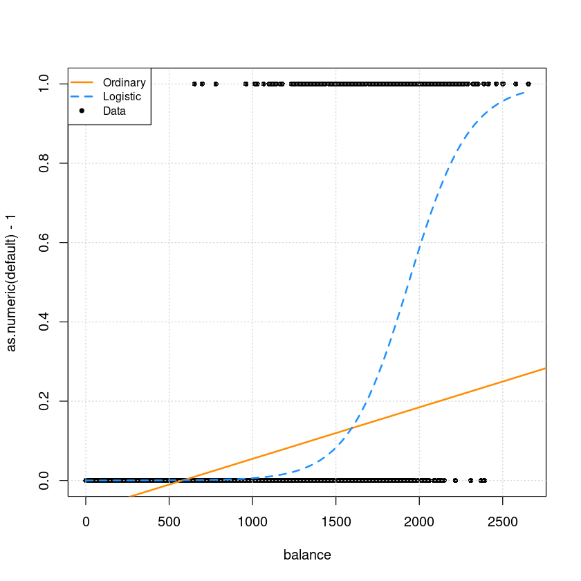
Predict
predict(glm.fits, data.frame(balance=2000)) #type='link' : default
1: 0.346503247961301
- 위의 값은 \(log\dfrac{p(x)}{1-p(x)}\)값
predict(glm.fits, data.frame(balance=2000), type='response')
1: 0.585769369615381
type = 'response'해야 \(p(x)\)값을 구할 수 있음.
y_2000 <- predict(glm.fits, newdata = data.frame(balance=2000), type='response');y_2000
1: 0.585769369615381
- $P(Default = “Yes” | Balance = 2000) = 0.585769369615381 $
y_1000 <- predict(glm.fits, newdata = data.frame(balance=1000), type='response');y_1000
1: 0.00575214508582045
par(mfrow=c(1,1))
plot(as.numeric(default)-1 ~ balance,data = Default,
     ylab = "Probability of Default" ,
     pch=16, cex=0.8, type='n')

curve(predict(glm.fits,data.frame(balance=x), type = "response"),
       add = TRUE, col = "dodgerblue", lwd=2)

lines(c(0, 2000),c(y_2000, y_2000), lty=2)
lines(c(2000, 2000),c(0, y_2000), lty=2)
points(2000, y_2000, col='red', cex=1, pch=16)

lines(c(0, 1000),c(y_1000, y_1000), lty=2)
lines(c(1000, 1000),c(0, y_1000), lty=2)
points(1000, y_1000, col='red', cex=1, pch=16)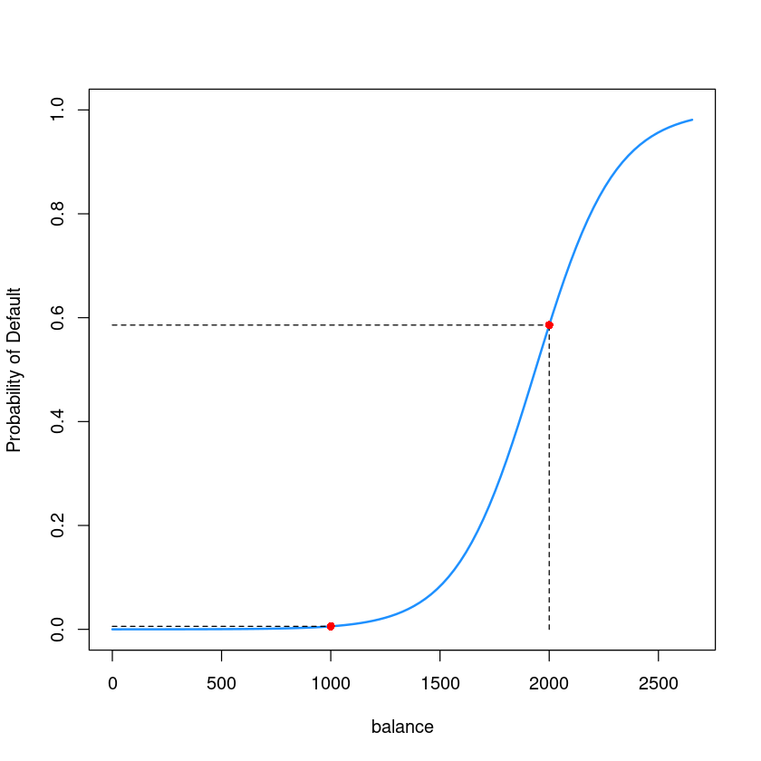
Confidence Interval
summary(glm.fits)
Call:
glm(formula = default ~ balance, family = binomial, data = Default)

Deviance Residuals:
    Min       1Q   Median       3Q      Max
-2.2697  -0.1465  -0.0589  -0.0221   3.7589

Coefficients:
              Estimate Std. Error z value Pr(>|z|)
(Intercept) -1.065e+01  3.612e-01  -29.49   <2e-16 ***
balance      5.499e-03  2.204e-04   24.95   <2e-16 ***
---
Signif. codes:  0 ‘***’ 0.001 ‘**’ 0.01 ‘*’ 0.05 ‘.’ 0.1 ‘ ’ 1

(Dispersion parameter for binomial family taken to be 1)

    Null deviance: 2920.6  on 9999  degrees of freedom
Residual deviance: 1596.5  on 9998  degrees of freedom
AIC: 1600.5

Number of Fisher Scoring iterations: 8- 95% CI : \(\hat \beta_1 \pm z_{0.025} s.e(\hat \beta_1)\)
- 방법1
confint(glm.fits, level = 0.95)Waiting for profiling to be done...
| 2.5 % | 97.5 % | |
|---|---|---|
| (Intercept) | -11.383288936 | -9.966565064 |
| balance | 0.005078926 | 0.005943365 |
- 방법2
summary(glm.fits)$coef| Estimate | Std. Error | z value | Pr(>|z|) | |
|---|---|---|---|---|
| (Intercept) | -10.651330614 | 0.3611573721 | -29.49221 | 3.623124e-191 |
| balance | 0.005498917 | 0.0002203702 | 24.95309 | 1.976602e-137 |
summary(glm.fits)$coef[2,1] + qnorm(0.975)*summary(glm.fits)$coef[2,2]
0.00593083451913757
summary(glm.fits)$coef[2,1] - qnorm(0.975)*summary(glm.fits)$coef[2,2]
0.00506699934268553
Classification
로지스틱은 분류모형에 해당
\(P(y=1|x) > 0.5 \rightarrow\) Default \(\hat y=1\)
\(P(y=1|x) \leq 0.5 \rightarrow\) Default \(\hat y=0\)
로 바꾸면 classification이 된다. 그럼 저렇게 0.5와 같은 기준값 (\(cut-off\))를 뭘로 정할까?
fitted.default.prob <- predict(glm.fits, type='response')
head(fitted.default.prob)- 1
- 0.00130567967421633
- 2
- 0.00211259491358475
- 3
- 0.00859474053900645
- 4
- 0.000434436819304936
- 5
- 0.00177695737814425
- 6
- 0.00370415282222879
class.default <- ifelse(fitted.default.prob > 0.5, 'Yes', "No")
head(class.default)- 1
- 'No'
- 2
- 'No'
- 3
- 'No'
- 4
- 'No'
- 5
- 'No'
- 6
- 'No'
table(Default$default, class.default) class.default
No Yes
No 9625 42
Yes 233 100왼쪽이 실제!
정분류율은 0.9725
class.default <- ifelse(fitted.default.prob > 0.3, 'Yes', "No")
head(class.default)- 1
- 'No'
- 2
- 'No'
- 3
- 'No'
- 4
- 'No'
- 5
- 'No'
- 6
- 'No'
table(Default$default, class.default) class.default
No Yes
No 9520 147
Yes 166 167